Jet Pump Design Basics
1. Introduction
Many sample datasets in SNAP demonstrate jet pumps. This tutorial assumes familiarity with hydraulic pumping concepts, jet-pump operation, and jet-pump size designations. A short Jet-Pump Primer is summarized here. For more depth, see:
- “Jet Pumping Oil Wells” by Hal Petrie, Phil Wilson, and Eddie Smart (World Oil, Nov 1983–Jan 1984).
- SPE Petroleum Engineering Handbook, Chapter 6 (hydraulic pumping). SNAP’s jet-pump design algorithms are based on this chapter.
Model Basis & References
The equations in the World Oil series were tailored for handheld calculators. SNAP implements computer-oriented algorithms derived from the SPE Petroleum Engineering Handbook, with additional empirical performance relations and corrections.
2. Jet-Pump Performance Theory
SNAP’s jet-pump performance relations are built from experimental nozzle and throat curves from water tests, with corrections for field conditions.
-
Power-fluid property handling
- Nozzle Reynolds number is high, so only specific gravity correction is applied when oil is the power fluid.
- Throat Reynolds number varies with rate and viscosity, so a produced-fluid viscosity correction is included, based on Amoco Research heavy-oil tests in the range 700 to 1900 cP.
-
Density and free gas effects
- Performance corrections account for density differences between power and produced fluids.
- Free gas is treated as additional liquid with a gas-interference factor, so the average density reflects free gas effects.
-
System hydraulics
- PVT and temperature along the well
SNAP computes specific gravity, viscosity, shrinkage, gas solubility, and formation volume factors at the appropriate depths using a linear surface-to-pump temperature gradient. In high-temperature, low-pressure conditions, steam vaporization is possible. Steam is modeled as a low-density water phase, not as a gas. - Friction and multiphase options
Power-fluid friction is computed for the selected tubing size and fluid properties using the full SNAP hydraulics and PVT suite. Earlier KOBE 4.1 programs used the Orkiszewski correlation for gassy returns. SNAP integrates full multiphase hydraulics instead of a single correlation.
- PVT and temperature along the well
-
Cavitation limit
- For each pump intake pressure, SNAP computes a cavitation limit which is the maximum flow at that intake pressure. Operating near this limit risks cavitation erosion and degraded performance.
- Cavitation logic assumes choked flow for free gas and corrects temperature using steam-table values.
Nozzle and Throat Geometry Families
- KOBE flow areas scale by .
- OILMASTER flow areas scale by .
- F vs E: F uses the same area ratio as E but with the World Oil curve instead of the KOBE curve.
- The same nozzle and throat sizes can be used in many assemblies. If catalog size and flow limits are respected, no extra pressure-drop corrections for different assemblies are needed.
2.1. Area Ratio Nomenclature (Y, X, A, B, C, D, E, F)
- Area ratio = nozzle flow area divided by throat flow area.
- A ratio: nozzle and throat have the same size number (example: 7-A is size-7 nozzle with size-7 throat).
- Increasing throat size with a fixed nozzle gives B, C, D, E, F (example: 7-C is size-7 nozzle with size-9 throat).
- X and Y ratios use smaller throats than A for the same nozzle.
Performance trends:
- As throat size increases (A to B to C to D to E to F): larger annular area gives higher potential production at a given , but less discharge head due to increased shear and mixing losses.
- As throat size decreases (A to X to Y): smaller annular area gives lower production, but greater discharge head from improved pressure recovery.
Capacity vs. Head Trade-off
Bigger throats raise capacity at the expense of discharge head. Smaller throats do the opposite. The best ratio depends on target rate, available power-fluid pressure, friction, and cavitation margin.
High-GOR modeling update:
SNAP includes improvements that correct high-GOR issues documented in the TRICO 4.1 jet-pump program.
3. Design Hints & Workflow (from the Trico Jet-Pump Manual)
- Horsepower (HP) constraint first. Try a couple of nozzle sizes to find the largest that fits the HP limit for the given depth and pump-intake pressure.
- Optimize area ratio for a chosen nozzle. For fixed power-fluid pressure and intake pressure, sweep ratios (A, B, …) to maximize production.
- Operating pressure vs. ratio. Larger throats (higher ratios) often require higher operating pressure (weaker pressure recovery). But if power-fluid friction is significant, a larger ratio + smaller nozzle can reduce overall surface pressure.
- General efficiency rule. Use the smallest nozzle that avoids cavitation while operating at the highest feasible power-fluid pressure (minimizes power-fluid loading).
- Example: 8B and 9A share the same throat size. 8B has more annular area for cavitation and may need less power fluid at the same operating pressure. Although B typically raises operating pressure, reduced power-fluid and return friction can offset it. Always compare cases.
- Discharge-pressure sensitivity. Roughly +3–5 psig in power-fluid pressure is needed to maintain performance per +1 psig rise in discharge pressure (more sensitive at higher ratios).
- Return GLR (from mixing power fluid with production) influences discharge pressure. A smaller nozzle can increase GLR, lower discharge pressure, and enable a larger ratio pump.
- Deep wells (~>6000 ft). Oil power fluid often performs better than water due to lower hydrostatic head. Water can “load up” the return column and stall the pump.
- Return conduit size matters in multiphase. With no gas, larger return conduit lowers discharge pressure; with gas, flow-regime changes can create an optimal size instead of “bigger is better.”
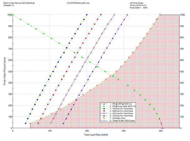
- Find the operating point by intersection. SNAP calculates a matrix of pump curves vs. power-fluid pressures. The well’s IPR intersects these pump curves to give operating points.
How SNAP Picks the Operating Point
On each pump-performance plot, overlay one or more well IPR curves. The intersection with a selected power-fluid pressure curve defines the predicted operating rate/pressures.
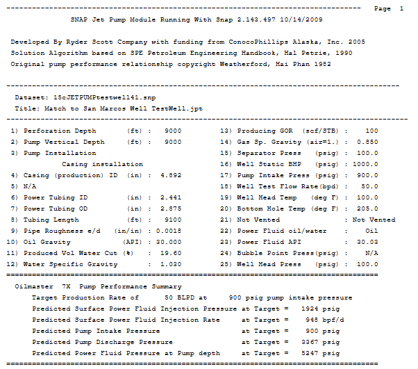
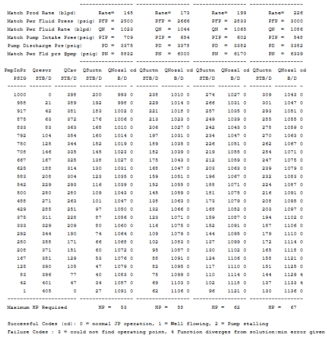
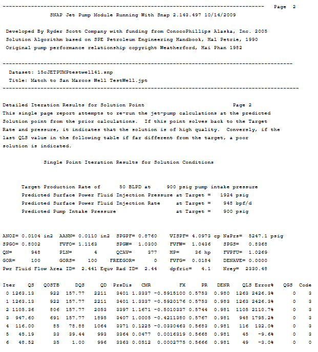
4. Sample Output Plot
5. Sample Jet-Pump Output Report