General Tutorial
The SNAP tutorial gives step-by-step instructions for creating a SNAP project. The tour uses the SNAP Default Dataset.SNP file that ships with SNAP. Working through the tutorial is an excellent way to become proficient with SNAP.
1. Beginning the SNAP Tutorial
We will begin by starting SNAP. If you have not yet installed SNAP, please do so.
-
Double-click the SNAP icon. On Windows you can also use Start >> Programs >> SNAP to open the program.

-
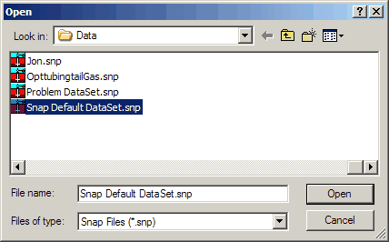
Choose File >> Open Dataset. The Open Dataset dialog appears.
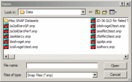
-
In the Open Dataset dialog, select SNAP Default Dataset.SNP, then click Open.
2. General Project Definition
Open the General Project Definition dialog by clicking General on the schematic.
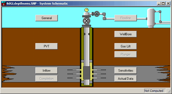
You can also select General from the toolbar using this button: 
You will see:
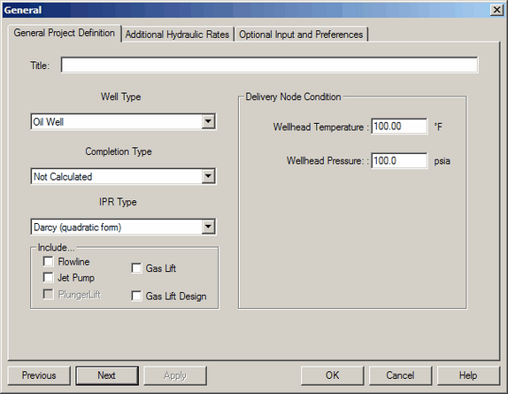
In this dialog you can name your dataset, indicate whether the primary phase is oil or gas, select an IPR type, define system temperatures and pressures, and set other conditions.
2.1. Well Type
SNAP performs calculations for:
- Oil Well
- Gas Well
- Water Injector
- Gas Injector
2.2. Completion Type
The Completion Type depends on the IPR chosen for evaluation. Options include:
- Not Calculated
- Cased/Gravel Packed
- Perforated
2.3. IPR Type
Online Help explains each IPR Type in the Inflow Reservoir and Well Data sections. IPR equations available in SNAP include:
- Darcy's Law
- Vogel's Method with Reservoir Data
- Vogel's from One Rate Test
- Vogel's from Two Rate Test
- Fetkovich from Multipoint Test
- Conventional Flow-After-Flow Test
- Isochronal Test
- Modified Isochronal Test
- Fetkovich from C and N
- Constant Productivity Index
- Babu & Odeh Horizontal Well Model
- Fractured Well Model
- Quadratic Flow Equation
- Back Pressure C and N
2.4. General Project Definition Exercise
- Click General on the SNAP schematic to open General Project Definition.
- For IPR Type, select Vogel's Method with Reservoir Data.
-
Click the Optional Hydraulic Rates tab. Enter flow rates of interest; these appear as symbols on the IPR curve(s) and Click OK.
# Flow rate #1 1200 #2 1400 #3 1600 #4 1800 #5 2000 -
Return to General Project Definition by clicking General again. Click Next to proceed to the PVT dialog.
You can also access PVT from the toolbar:
Panel Availability
Making changes early can activate or remove certain input panels. Make sure you have data in the correct locations and do not leave required dialogs empty.
3. PVT Properties
The PVT Properties dialog enables you to enter basic reservoir pressure, volume, and temperature data to describe a reservoir's fluid. PVT parameters are pressure dependent and change with time.
This dialog changes slightly depending on whether you select an oil well or a gas well.
- Oil well: Correlations are available for solution GOR, formation volume factor (Bo), and oil viscosity. See Help >> Input Panels >> PVT Properties for guidance on which correlation to use.
- Gas well: No correlations are available; the Oil API Gravity and Water Specific Gravity fields are deactivated.
3.1. PVT Exercise
- The PVT window should be displayed from where we left off. If not, click the PVT button on the toolbar.

- Review the drop-down lists for Solution Gas/Oil Ratio, Oil Formation Volume, and Oil Viscosity. Leave the original selections.
- Click Next to proceed to the Inflow Properties dialog.
4. Inflow Properties
The Inflow dialog is specific to the IPR selected in General Project Definition. For this tour the IPR is Vogel's Method with Reservoir Data. Use this dialog to enter data for the single- and multi-point correlations used in pressure drop calculations.
Access it from the toolbar:  , by clicking Inflow on the schematic, or via Inputs >> Inflow.
4.1. Inflow Properties Exercise
- Start with this dialog:
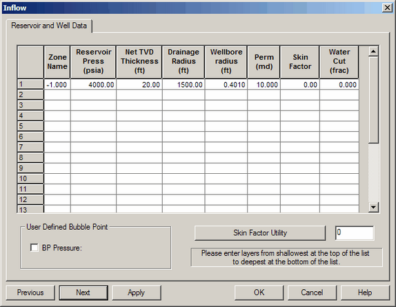
- Change Reservoir Pressure to 3000 psi.
- Click Next to proceed to the Flowline Geometry dialog. If you reach the Wellbore page, go back to General and check Include >> Flowline, then click Flowline on the schematic.
5. Completion Data
The Completion Data dialog is not active because the selected IPR does not require Completion Type input. When active, you can fine-tune completion algorithms and model up to five commingled zones for Darcy's Law or Vogel's with reservoir data.
6. Flowline Geometry
The total length of the flowline is described using pipe diameter changes, non-linear temperature profiles, and segments that describe the flowline profile. You begin at the separator and work toward the wellhead. Because component elevations affect performance, SNAP offers three geometry methods:
- ML (Measured Length) vs Angle
- ML vs Elevation
- Elevation vs Angle
You can choose from the following five hydraulic correlations:
- Dukler
- Beggs & Brill
- Mukherjee & Brill
- Dukler & Eaton
- Minami-Beggs-Brill
6.1. Flowline Geometry Exercise
- If Flowline Geometry is not displayed, select Flowline from the toolbar.
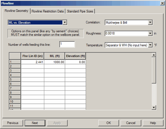
- In the Flow Line ID (in) column, click the value 2.441.
- Click the Standard Pipe Sizes tab to open Dimensions of Standard Tubing.
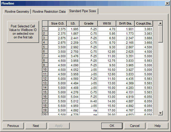
- Locate and click the row with ID = 1.995 for P-110 Grade.
- Click OK to return to Flowline Geometry. The flowline ID updates automatically.
7. Wellbore Geometry
Wellbore geometry can be a single tubing string or multiple strings depicted as segments that describe the wellbore. You begin at the wellhead and end at the bottom of the hole. You can model annular or tubular flow.
Hydraulic correlations include Hagedorn & Brown, Orkiszewski, Duns & Ros, Aziz, Beggs & Brill, Gray, Mona, Modified Gray, Duns-Ros-Gray, Mechanistic, and Cullender-Smith. Click Hydraulics Correlation to open the Correlation Advisor.
7.1. Wellbore Geometry Exercise
- If Wellbore Geometry is not displayed, select Wellbore from the toolbar or click Wellbore on the schematic.
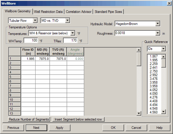
- Click Correlation Advisor to open it.
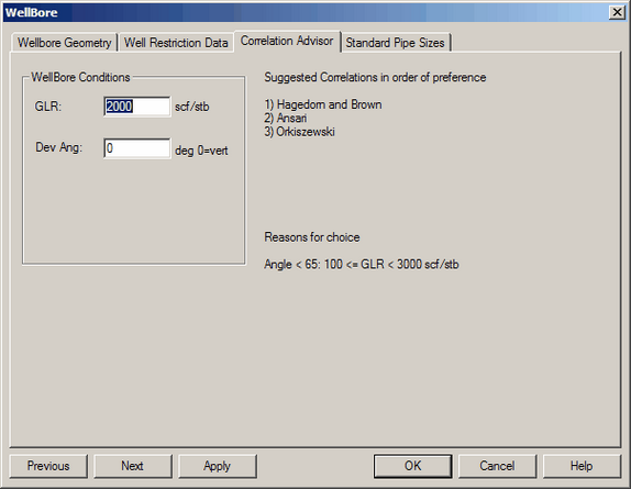
- Click Update to view Suggested Correlations based on your inputs. Choose the one that works best when you return to Wellbore Geometry.
- Click Done to exit the advisor.
- Click Next to proceed to Sensitivities.
8. Gas Lift
If your well uses gas lift, provide gas lift characteristics for an accurate analysis. SNAP enables Gas Lift only if you select Include Gas Lift in General Project Definition.
Gas Lift Not Considered in This Tour
For this walk-through, Gas Lift is not considered, so the option remains inactive in General Project Definition.
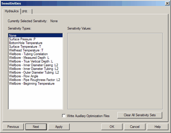
9. Sensitivities for Calculations
Use Sensitivities to vary system parameters and evaluate their effects on IPR and hydraulics. Each effect appears as an additional curve on the results graph when you run calculations. SNAP hides sensitivities that are not applicable. You can enter Tubing, Reservoir, or Combined sensitivities.
9.1. Sensitivities Exercise
- If the Sensitivities dialog is not displayed, click the Sensitivities button on the toolbar.
- Change the flowline pressures to match your desired cases, then click OK to save and return.
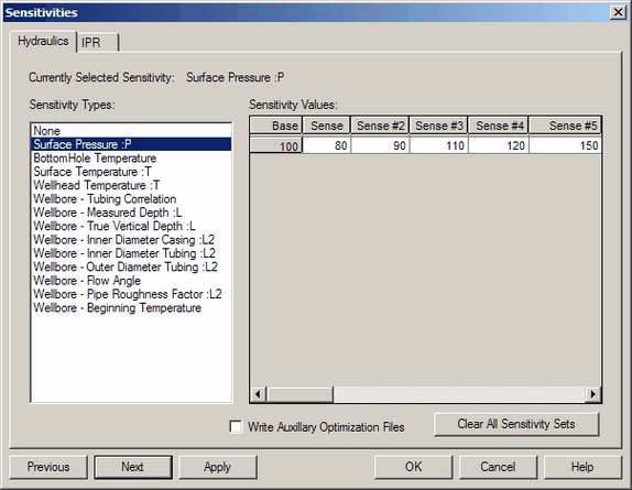
- Click X to close Sensitivities.
10. Calculating the Nodal System
After entering all data, calculate the nodal analysis. You can calculate the entire analysis, only the IPR curve set, or only the hydraulic curves.
10.1. Calculation Exercise
- Choose Calculate >> Calculate All to compute both IPR and hydraulics.
- View the resulting plot. Observe the sensitivity curves for IPR and hydraulics and the symbol locations for Optional Hydraulic Flowrates, Minimum Lift Rate, and Minimum Flow Rate.
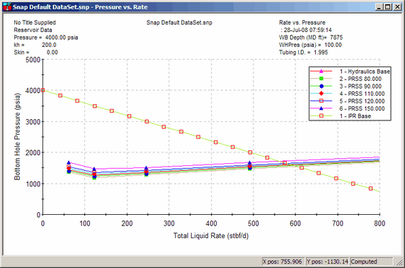
11. Plots
After entering and editing data, you can generate, manipulate, and print IPR, hydraulics, and system plots. You can also generate a gradient plot for the baseline and optional hydraulic flowrates.
When you generate a plot, it opens in a Plot Viewer window. Three menu items appear:
- Edit — customize layout, colors, fonts, and other printing characteristics
- Tools — zoom in or out and view a project summary
- Plots — view graphical representations of calculated values
SNAP can generate these plot types:
- Rate vs Reservoir Pressure
- BH Pressure vs Reservoir Pressure
- Rate vs Flowline Pressure
- BH Pressure vs Flowline Pressure
- Gradient Curve
11.1. Plots Exercise
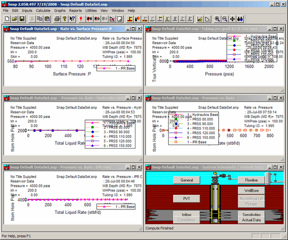
- Choose Graphs >> Sensitivity Results >> Rate vs Surface Pressure. The Surface Pressure plot appears.
- Open the next four plots the same way. Each plot opens in the application window.
- Choose Window >> Tile to view all plots together.
12. Report Format
SNAP also generates reports after you run calculations.
12.1. Report Exercise
- Choose Reports >> Summary to display a summary report. Or choose Reports >> Gradient for a gradient report.
- After viewing the report, close the window.
13. Exit SNAP
Choose File >> Exit.